MLGroup29
Multi-Label Genre Classification of Movies From Their Posters
Drew Hatcher, Jahin Ahmed, Nikhil Rajan, Parker Bryant, and Zach Hussin
Problem Statement
Movie posters can provide a lot of information for people going to see movies. Apart from the cast and crew, visual features and structural cues are guiding factors in classifying a movie genre. However since the idea for posters was first conceived, we have have a vast range of styles, ranging anywhere from minimalist graphic design to intricate composite photographs.To better understand the design choices behind movie posters, our project aims to create a classification model that is able to predict a movie’s genre based on features that it’s poster possesses. Prediction tools of this nature can be applied to areas such as detection of unwanted image content on platforms, categorising videos based on their thumbnails, and perhaps falicitating data for a discrinimator neutral network of a GANs in order to verfiy fake content.
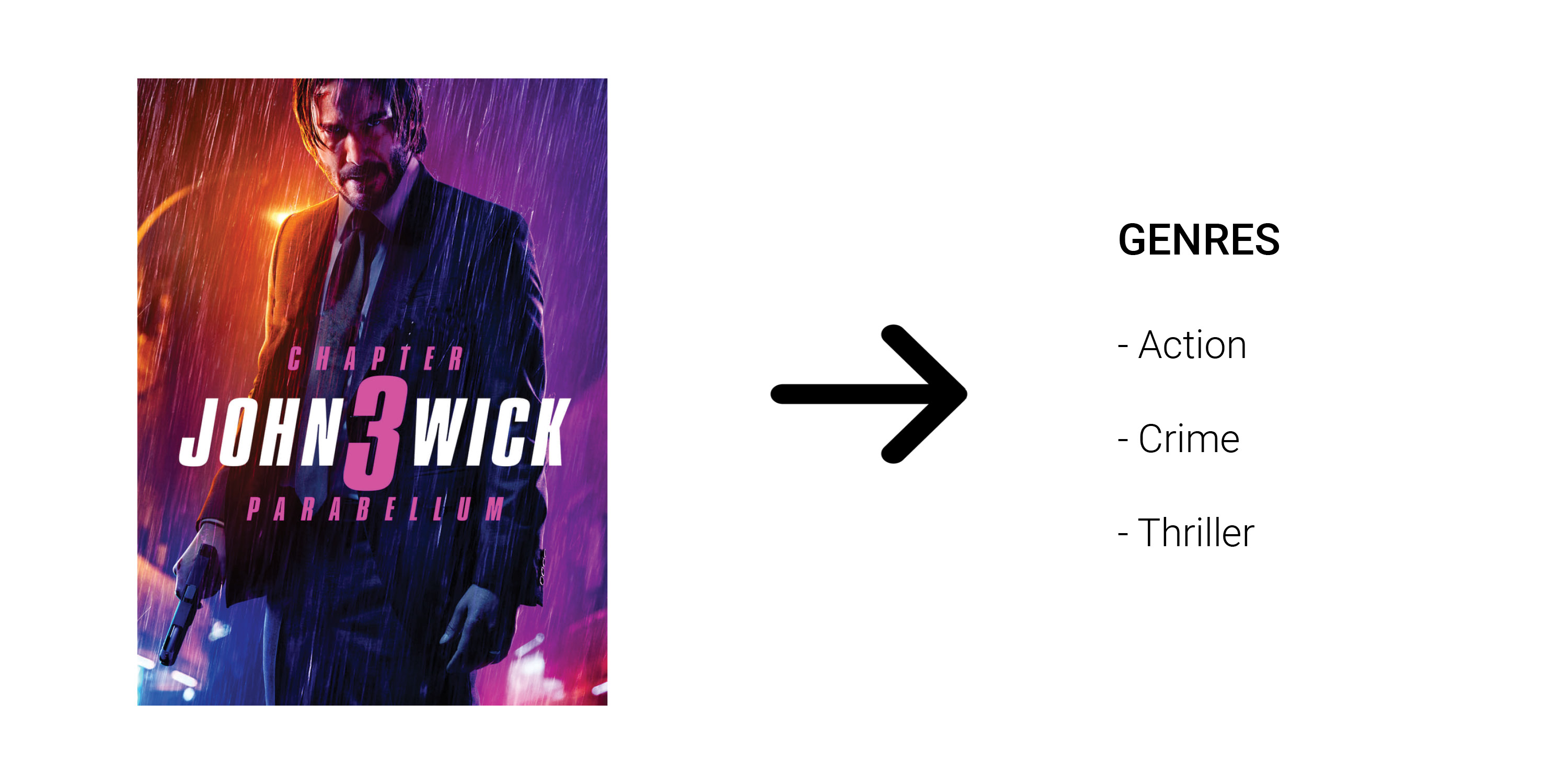 Figure 1
Approach Overview
Our goal in this project was to create a supervised learning model that would accurately classify a movie’s genre based on its poster. In order to do this, we needed to obtain genre classification and poster images for a significant amount of movies. We found a dataset of movie data that was harvested from TMDB and from that large dataset, we preprocessed the data to cut away unnecessary information and to fit the parameters of our model. From our preprocessed data, we created a smaller subset of the data in order to test potential models with efficiency. After extensive research, it was clear that convolutional neural networks are the most used and effective supervised learning technique for classifying images. Other methods including dimensionality reduction algorithms like PCA were found to have certain pitfalls when dealing with data like ours in which there is a high likelihood that our dataset will be imbalanced with more genres like drama and comedy than western films, as shown in the dataset below. Implementing these methods would train the model to find those genres better, rather than being a good classifier for all genres.
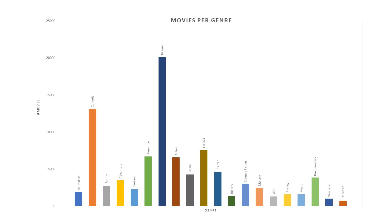 Figure 2
Finding this, we decided to create a cnn and then run experiments changing a single variable at a time to hone in on the overall most efficient and accurate classification model.
Data Collection
After locking in on our problem, the next step in solving our problem was to find data around and relating to our project that we could use to build a model. Because of the specificity of our problem, there wasn’t a bulk of readily available data from big name sources, so we turned to Kaggle, which is an online community dedicated to machine learning initiatives where a wide variety of datasets are collected and made public to the community. From Kaggle, we were able to find a catch all dataset for a set of over 40,000 movies. This dataset, called “The Movies Dataset” is described as an ensemble of data collected from TMDB using their public API [1]. The dataset has almost 68,000 downloads and a usablity rating of 8.2. We decided the dataset would be a great fit for our problem based on the credibility of the source, the categorical data collected, and the sheer size of the set.
The dataset we used can be found here: The Movies Dataset
Preprocessing
When deciding what dataset to use, we realized there would be a tradeoff between the quality of the data that we acquired and the time it would take to preprocess that data. Choosing to use The Movies Dataset gave us the highest quality and quality of data, but came at the cost of a significant amount of data preprocessing before we could even start building a model. We still decided upon using the dataset because we realized building a model with a low quality and quantity of data would give us an unreliable model, which in the end isn’t worth the trouble.
Filtering Unuseful Information
From The Movies Dataset, we were able to narrow our usage to only movie metadata, but this still left us with an overwhelming amount of unnesessary information. The movie metadata was a csv file of over 45,000 columns and 24 rows. Each of these rows corresponded to an attribute about a movie, and here is a example of a row in that csv:
| adult | belongs_to_collection | budget | genres | homepage | id | imdb_id | original_language | original_title | overview | popularity | poster_path | production_companies | production_countries | release_date | revenue | runtime | spoken_languages | status | tagline | title | video | vote_average | vote_count |
|---|---|---|---|---|---|---|---|---|---|---|---|---|---|---|---|---|---|---|---|---|---|---|---|
| FALSE | {'id': 10194, 'name': 'Toy Story Collection', 'poster_path': '/7G9915LfUQ2lVfwMEEhDsn3kT4B.jpg', 'backdrop_path': '/9FBwqcd9IRruEDUrTdcaafOMKUq.jpg'} |
30000000 | [{'id': 16, 'name': 'Animation'}, {'id': 35, 'name': 'Comedy'}, {'id': 10751, 'name': 'Family'}] |
http://toystory.disney.com/toy-story |
862 | tt0114709 | en | Toy Story | Led by Woody, Andy's toys live happily in his room until... |
21.946943 | /rhIRbceoE9lR4veEXuwCC2wARtG.jpg |
[{'name': 'Pixar Animation Studios', 'id': 3}] |
[{'iso_3166_1': 'US', 'name': 'United States of America'}] |
10/30/1995 | 373554033 | 81 | [{'iso_639_1': 'en', 'name': 'English'}] |
Released | N/A | Toy Story | FALSE | 7.7 | 5415 |
Obviously a large chunk of this data was unrelated and took up a lot of space, which would complicate things down the road trying to build the model. So immediately, our first thought was to create a new csv file that we could refer to later, that only contained the relevant movie attributes. Given our problem statement, we narrowed our neccessary or wanted attributes down to ‘id’, ‘title’, ‘genre’, and ‘posterpath’. We kept the id column as it was needed to connect a movie to it’s poster and genre. We found the title was useful to as it allowed us to test our data processing and ensure the data was still associated with the correct movie. Genre was obviously needed in order to train and test our model using the proper genres, and posterpath was just as important as it gave us access to the images we were analyzing. Afterwards, our data looked something like this:
| id | title | genres | posterpath |
|---|---|---|---|
| 862 | Toy Story | [{'id': 16, 'name': 'Animation'}, {'id': 35, 'name': 'Comedy'}, {'id': 10751, 'name': 'Family'}] |
/rhIRbceoE9lR4veEXuwCC2wARtG.jpg |
Removing Invalid Data
Once we had narrowed our dataset to only the essential information, we were able to closely analyze each piece of data to ensure its validity with higher efficiency. While the dataset is credible, we realized that since the dataset was created, many things could have changed, and even then, it’s possible that not every movie’s data was in good condition to be analyzed. Because of this, we came up with some minimum conditions for us to keep the data. The first of which was that each movie must have at least 1 associated genre, and a path to a poster image. To meet this restraint, we looped through the entire processed lists of movie and deleted any row that had a null posterpath or genre. This simple filtering alone dropeed around 5000 rows from dataset.
While this restriction did most of the dirty work, there was still the possibility that some data was invalid as not all of the posterpaths mapped to a valid url with an image. To take care of this, when we collected our posters (detailed process described next), we were able to include checks that would make sure that not only the url was valid, but also that a proper jpg file could be created from that path. In doing this, we were able to collect the id of each movie that didn’t have a valid poster, and directly dropped these rows from our processed csv. With these conditions, we were confident that our data was cleansed enough to be reliable in training.
Binary Genre Conversion
In order to create a model to train, our genre’s must be in a processable and stardardized format. Our genres were currently being read as a string of seemingly random characters that doesn’t have any meaning to a neural network. To fix this problem, we decided to compose a list of all of the genres represented by our data, which turned out to only 20 genres. This required converting the string genre’s into json objects and looping through to find unique genre values. We created a column for each genre, and looped through each row in our data, marking the respective columns with a 1 if the movie was of that genre and a 0 if not. Here is an example of how the genre’s were classified for each movie:
| id | title | genres | posterpath | Animation | Comedy | Family | Adventure | Fantasy | Romance | Drama | Action | Crime | Thriller | Horror | History | Science Fiction | Mystery | War | Foreign | Music | Documentary | Western | TV Movie |
|---|---|---|---|---|---|---|---|---|---|---|---|---|---|---|---|---|---|---|---|---|---|---|---|
| 862 | Toy Story | [{'id': 16, 'name': 'Animation'}, {'id': 35, 'name': 'Comedy'}, {'id': 10751, 'name': 'Family'}] |
/rhIRbceoE9lR4veEXuwCC2wARtG.jpg |
1 | 1 | 1 | 0 | 0 | 0 | 0 | 0 | 0 | 0 | 0 | 0 | 0 | 0 | 0 | 0 | 0 | 0 | 0 | 0 |
Once the binary classification was complete, it was aparent that for our model, the title, posterpath, and genre columns would not be needed in our model, and thus, we dropped those rows from the csv file. This left the id’s of each movie corresponding to an index into the image numpy array, and columns of genre’s to classify the images.
Poster Collection
Because we were still working with over 40,000 images, we knew that obtaining the images would be both time and space intensive, so instead of trying to do this every time we trained, we decided to collect all of the posters and host them locally in a saved array. Before we could do this, we first had to create a script that would loop through each posterpath and retrieve the image associated with that movie. We then saved each image as a jpg named by their corresponding id in a directory dedicated to poster images. As we did this, we were also adding each image to a numpy array that was then saved locally with a size of over 16 GB. Having this array locally allowed us to refer directly to a certain element during training, which drastically increased the speed of our model.
Image Compression
Understanding what we knew about locally hosting images, in terms of overall time and space complexity, we had to decide on the proper size for images. Our poster paths were url extenstions that accessed images from TMDB’s web server. Using TMDB’s api, we found that we could pass in a few different values in our url parameters and get different size images. After discussing as a group, we agreed that the larger the image, the marginal increase in information is much lower than the marginal time and space required to compensate that large image. Thus we went with the smallest poster image, that still gave clear and distinguishable shapes, settling upon images with a width of 185 pixels for each image.
During our poster collection process, it came to our attention that there wasn’t a standard height for the images that we were collecting. This could cause problems in our convolutional neural network, because a standard size is required for the model, and even if it wasn’t, non standard data could throw off the results of our filtering in our convolutional layers. Thus, we decided in order to standardized our images, we would compress each image such that it’s height was also 185 pixels.
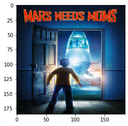 Figure 3
This way, shapes and details were still being captured similarly accross posters and it shouldn’t affect the performance of our network. To compress the images, we used a load image function that is a part of the tensorflow keras image preprocessing library. This function uses a nearest neighbor interpolation strategy that replaces a group of pixels with a single pixel based on neighboring pixels and the ratio of the new size to the original size. With our newly sized 185x185 images, we realized that any further dimensionality reduction was unnessesary and could be harmful to the accuracy of our model. We now had a 4D array of an approximate size (40000, 185, 185, 3) to use for our training, of which we split our
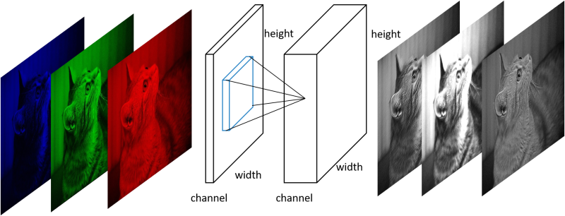 Figure 4 [2]
Building the Convolutional Neural Network
Using Google’s Tensorflow, we were able to build our neural network by supplying it the parameters we desired for our model. We decided to follow the structure of the Oxford Visual Geometry Group (VGG), as it is proven to have effective for image classfication, most notably winning ImageNet’s Large Scale Visual Recognition Challenge. The structure was obtained through a reigourous evalutaions of netowrks of increasing depth, showing that siginificant improvements can be seen by increasing the depth to 16-19 layers and using very small 3x3x1 filters for all convolutional layers to reduce the number of parameters[5].
Although we did not use their model as our framework, we built a Sequential model following the VGG-type structure, with the same filter sizes followed by a max pooling layer, which we repeated with doubling the number of filters when each layer was added. Additional parameters we believed to be appropriate based on the structure and other research included the use of the Rectified Linear Unit as activation, for all layers except the final one to avoid saturation (an issue when using the sigmoid function, a nonlinear activation function):
Expand Code
```model = Sequential() model.add(Conv2D(16, (3,3), activation='relu', input_shape = X_train[0].shape)) model.add(BatchNormalization()) model.add(MaxPool2D(2,2)) model.add(Dropout(0.3)) model.add(Conv2D(32, (3,3), activation='relu')) model.add(BatchNormalization()) model.add(MaxPool2D(2,2)) model.add(Dropout(0.3)) model.add(Conv2D(64, (3,3), activation='relu')) model.add(BatchNormalization()) model.add(MaxPool2D(2,2)) model.add(Dropout(0.4)) . . . . . model.add(Dense(20, activation='sigmoid')) ```
The final layer uses sigmoid to produce a 20-element vector (for the 20 different genres) with prediction values ranging from 0 to 1 for each output class. This is prefered to the softmax activation function as we have a multi-label classifier not a multi class classifier.
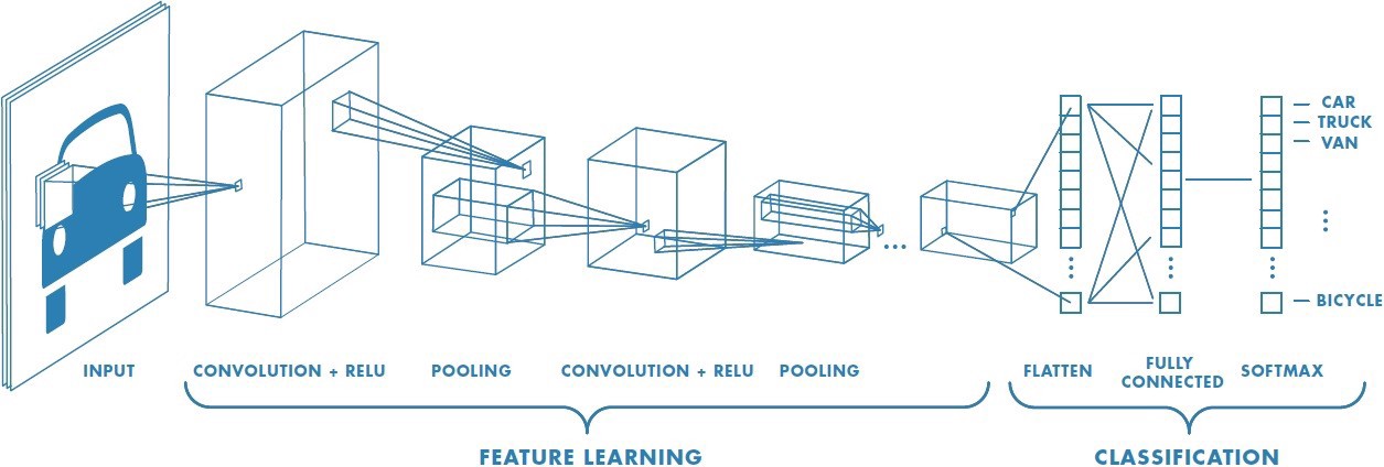 Figure 5 [4]
Finally our model is optimized using Tensorflow’s Adam Optimization algorithm, which is an extention of stochastic gradient decent, for reasons including speed of processing, more intuitive interpretation of the hyper-parameters, noise reduction, to name a few.
Adjusting our Model
Based on our understanding of Convolutional Neural Networks, we wanted to adjust the parameters and layers of our base model in order to achieve different results to learn about our model. Based on tensorflow.keras.conv2D, we analyzed each parameter including filter size, number of filters, activation, and manipulated those that we thought would have the most significant impact on our model [3].
- Original Model From Above
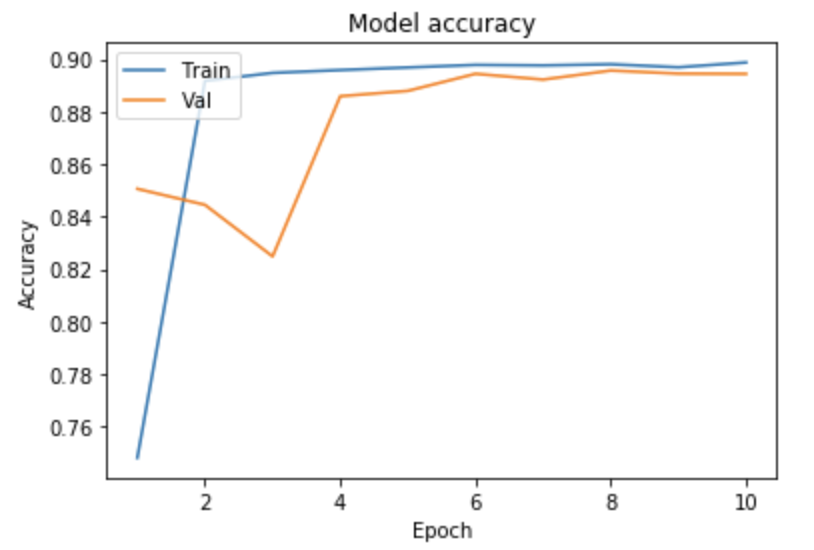
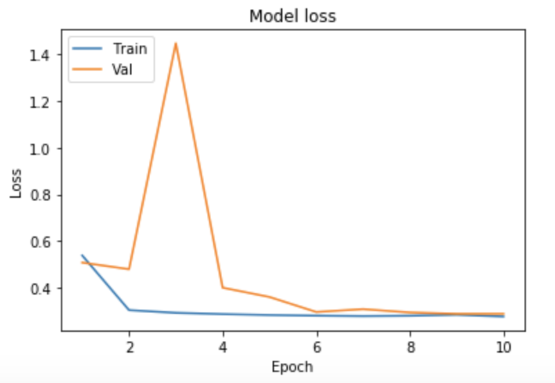
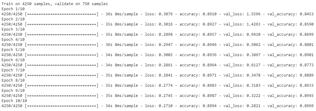
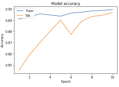
- 4 Convolutional Layers with 10 Epochs
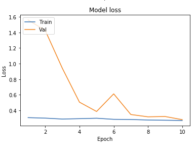
- 5 Epochs with 4 Convolutional Layers Using Adamax OptimizerAccuracy

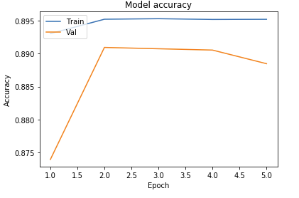
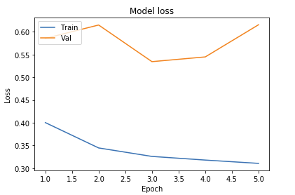
- Original with 5 x 5 Convolutional Filters
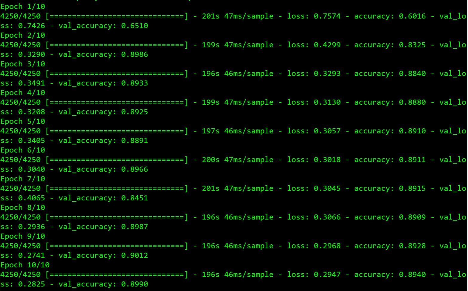
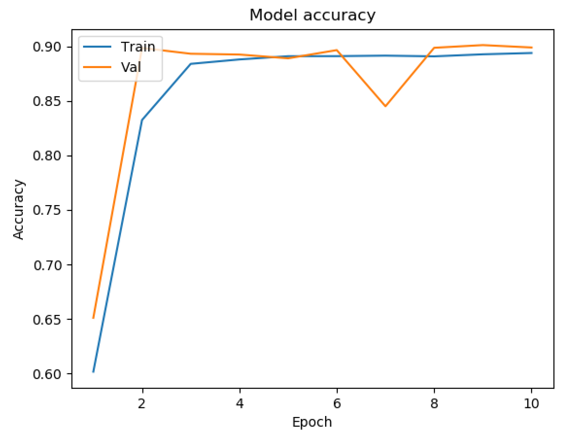
- 5 Epochs with 5 Layers

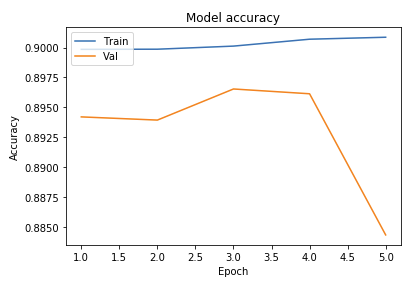
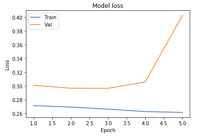
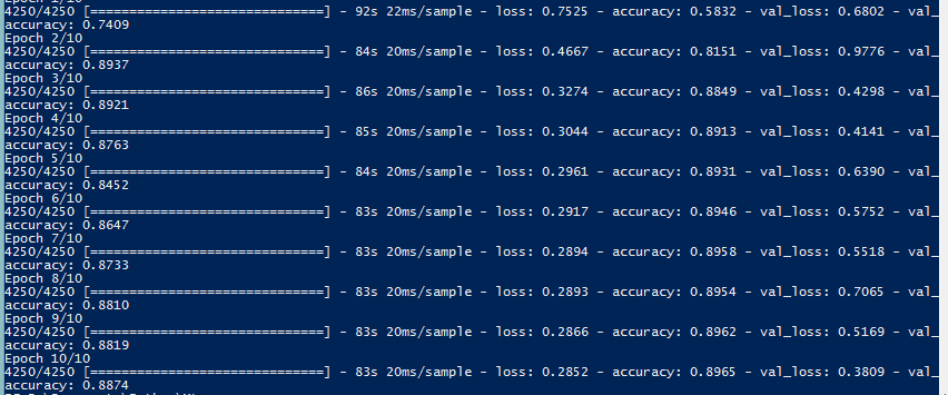
- 8 Conv2D Layers with 64 Filters
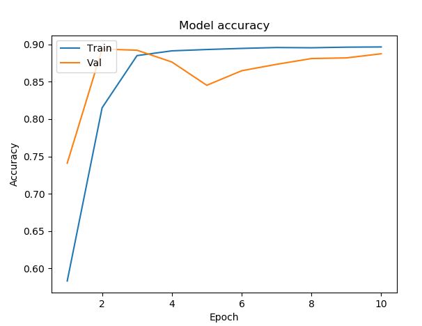
Model Testing Analysis
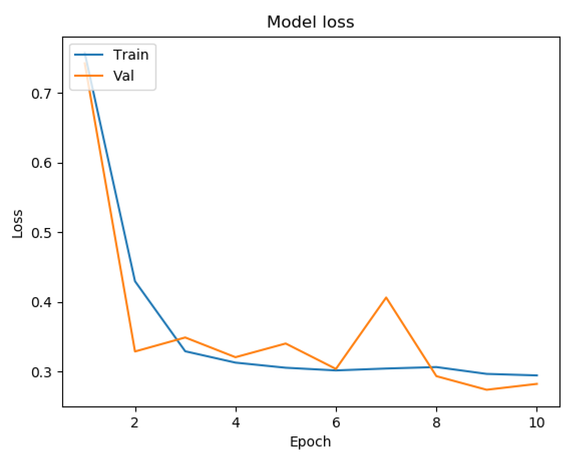
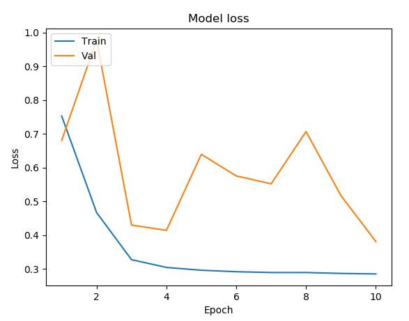
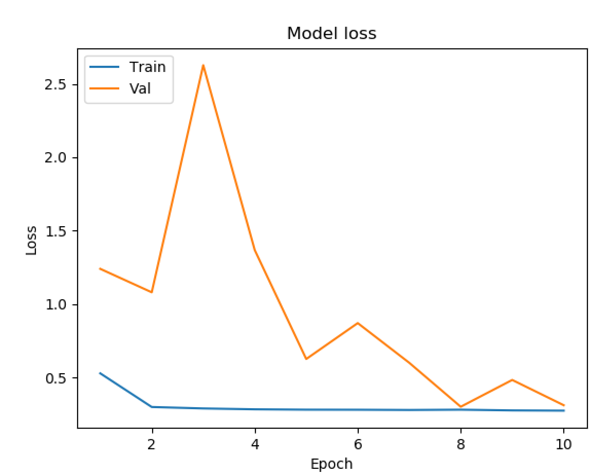
As seen above, we ran tests on multiple different models to determine what the best parameters of our model were. Our original base model performed well, having plateaued off at around 90 percent accuracy. For a first trial, we viewed this as a success, but wanted to see how much better we could do if we strayed from the norm slightly in different directions. Next we decided to test using 4 Convolutional Layers instead, which hit a loss of .27 and an accuracy of 89 percent. This showed that the final convolutional layer provided only the slightest bit of extra help, but very slim at that. We followed that by running 5 Epochs with 4 Convolutional Layers Using the Adamax Optimizer. 5 Epochs should theoretically have a lower accuracy, but with the Adamax Optimizer, the accuracy stayed very constant at around 89 percent again. We did see a spike in loss, upwards of .61, which isn’t as good as previous. Comparing this to other trials at around 5 epochs, the Adamax Optimizer didn’t seem to have much of an effect on our model. Next we ran the original trial with 5x5 convolutional filters instead of 3x3. Again, this modeled seemed to hit the 89.5 accuracy mark with a loss of .28, but it seemed that with the 5x5 filters, much fewer epochs were required for the accuracy and loss to begin to plateau. After this, we attempted to switch things up by only running 5 epochs on 5 Convolutional Layers, but no matter what we seemed to do, we still arrived at just above 89 percent accuracy again with a loss of 1. This loss was much greater than anything we’d had before, so we decided against this method completely. Finally we attempted to run 8 layers, each with 64 filters as a last attempt to adjust our model. Instead, we fell just shy of 89 percent with an adequate loss of .38.
After all of our trials, it seemed as if the more we strayed from our original model, the worse the loss became, while the accuracy failed to get any better. We found that adding more filters didn’t positively impact our model, while decreasing the number of filters didn’t negatively impact our model. Based on this, we are fairly confident that most of the genre determination can be made from the more basic and vague shapes instead of the more specific details. Knowing this could be very helpful in the future when deciding whether the space/time tradeoff is worth it when considering adding more filters to a network similar to ours. This information could also be used to hypothesize about how feeling is actually conveyed through images. In our testing, we also found that adding additional layers did little to help us, and after a certain point, more epochs were no longer helpful either. The one model that we saw might have potentioal was the original model but using a filter size of 5x5 instead of 3x3. Though this was an unexpected development, we decided to run with it as very few other models use 5x5 filters in this type of classification.
Final Results
Running with what seemed to be our best model from testing, we wanted to train the same model with a larger dataset. By doing this we were hoping that an increased number of movie data would produce a better training set, and in turn would increase our prediction accuracy.
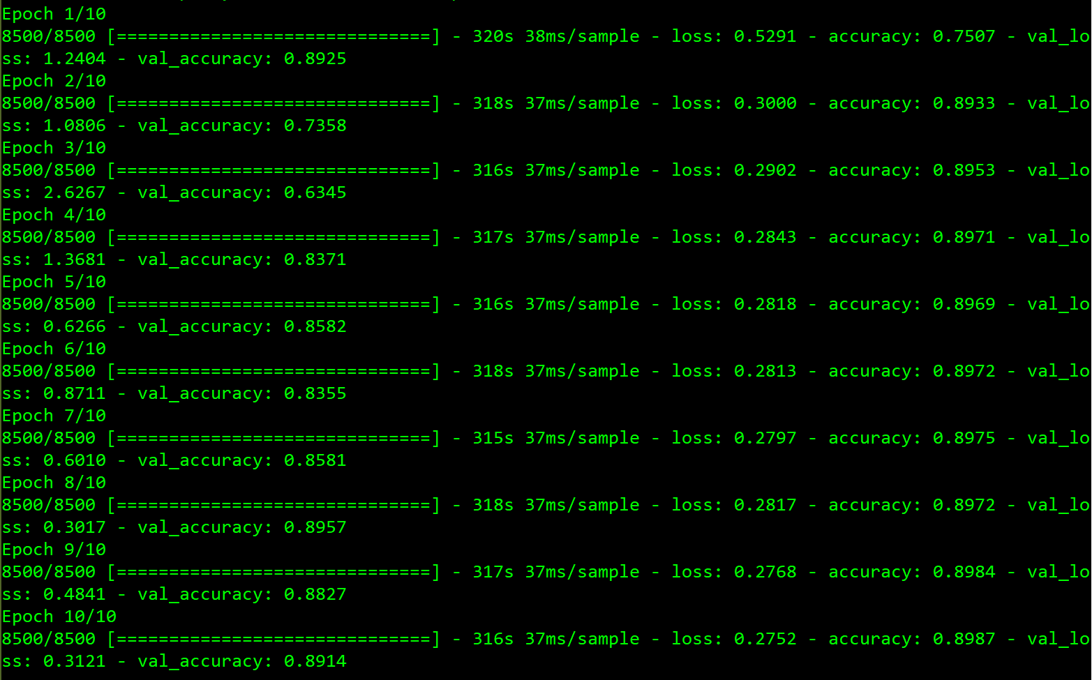
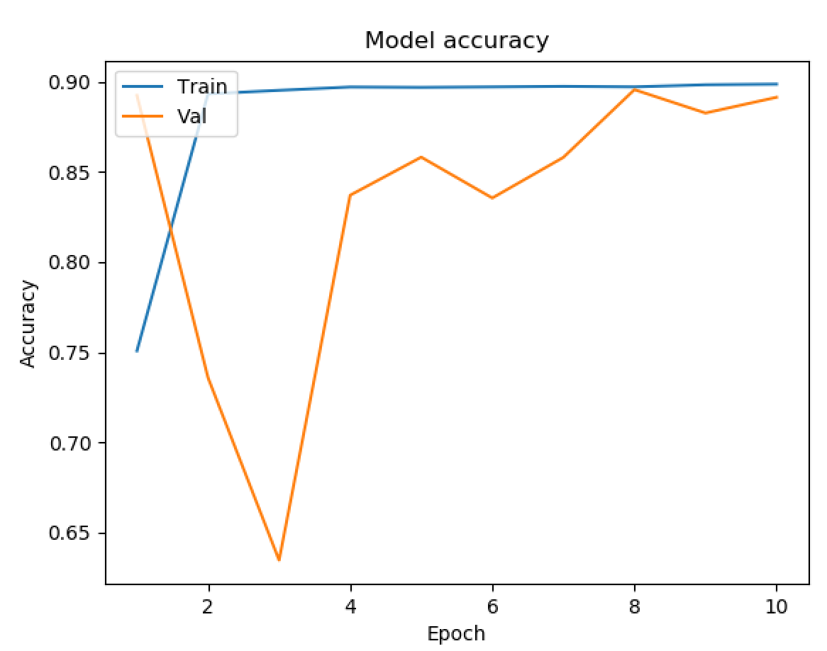
With our final model, we found that our accuracy was maxing out just shy of 90 percent, very similar to all of our trial models with less data. We also found that we only had a loss of 27.5 percent, which was about the best our training data got as well. From the final results, there wasn’t much evidence that an increased number of images changed the accuracy, or efficiency of our model, while being twice as slow. As such, we recommend training on a dataset of around 5,000 images as of now.
While our final results with a larger dataset didn’t garner better results, 90 percent accuracy with a 27.5 percent loss is a very successful model when considering multi valued classification with a total of 20 classes.
Evaluation of our approach with F-beta
Since our dataset does not have a balanced number of examples of each class, as shown in the Approach, nor do we perform binary or multi-class classification, an appropriate measure of the accuracy of our results was deemed to be the F-beta metric. This is related to the F1 score/measure, in which the average of recall and precision is calculated to find the harmonic mean. This is the prefered method of evaluating performance of an imbalanced dataset.
THe idea of postive and negative classes (for correct/incorrect model predictions) only make sense for a binary classification problem, and thus we need to introduce wieghts to how important recall is in comparison to precision, in that each class is compared in a one vs. all others manner.
A common weight that is used for these problems is 2, in which recall is valued twice as highly as precision. As we also care more about recall, we will also set beta = 2 since we want the model to be as accurate is possible. Thus we are looking for F-beta around 1 for our model, to reach the harmonic mean.
The results of the tests are as follows:
| Trial Specifications | F-beta Value |
|---|---|
| 5 Epochs, 4 layers, softmax activation | 0.890 |
| 5 Epochs, 5 layers, sigmoid activation | 0.844 |
| 5 Epochs, 4 layers, sigmoid activation | 0.890 |
| 10 Epochs, 4 layers, sigmoid activation | 0.895 |
| 5 Epochs, 4 layers, adamax optimization | 0.838 |
From the example of results above, we can see that the big factors of change were increasing the number of epochs and remaining with the sigmoid activation, which worked better for multi-label classification models. This can be taken a step further by changing the beta values for similar testing.
Possible Improvements Discussion
Looking at our results, there are a few things that could have negatively impacted the accuracy of our neural network. In reference to the graph of movies per genre seen in the approach overview section above (Figure 2), you can see that the number of movies per genre is not standardized. Because some genres such as Drama and Comedy have a disproportionate number of movies compared to the genres of say Westerns and History, our model is trained to classify more movies as such. While CNNs are better models at correcting for the imbalance of data, there will always be some disturbance. Because of this, if we fed a Western into our model, it has a higher chance of mislabeling it as such. In future studies, if we were able to stablize the number of movies per genre, we would likely get better predictions.
Another possible hinderance of our model is the size images that we are using. Because of space and time constraints, we decided to work with 185x185 pixel images, but this could have slightly decreased our model’s accuracy. The first reason is because we compressed multi sized portrait images into a standard square, which could have warped the shape of some posters in respect to other images, throwing off some of the filters we use in our convolutional layers. The second reason the image size is an issue is because some of our convolutional layers used a high amount of filters, which increasingly adds specificity to the filter. Because we are using lower quality images, filters with high specificity trying to identify precise shapes may not be able to classify these shapes as well. In turn, this could affect the probability that an image is of a certain genre, which could have led to slightly lower accuracies in our model. In the future, higher quality images can be used with the understanding that the model will take exponentially longer to train and test, and the memory required may be much harder to attain.
Conclusion
After analyzing our results, we were able to make significant progress on top of other attempts at solving the same problem. The size of our dataset gave us more information to work with, which led to more accurate classifications. But our convolutional neural network was also different than any we’ve seen thus far.
By intially following the VGG type structure, we were able to build off of an already great classifier. We took characteristics of that type of model and changing parameters we felt could yield better outcomes, and that proved to be the case from the results shown above. Our model classifies a genre correctly 9 out of 10 times, which is very good considering we are using multiple genres per movie.
The reason our solution is important is because it has a implication for real world use. It provides evidence that there are certain features that are associated with different genres, and with that, different emotions. This is very valuable information for designers aiming to attract the correct target audience by appealing to their emotions. In the future, this tool could be slightly modified to grade how well a movie poster defines its movie, which could help movie advertisers as a whole. Aside from that fact, this classification could further be broadened to classify genres of not only movies based on posters but possibly even the genres of movies based on scenes within the movie, or music genre based on album cover. The practical applications for this type of model is a wide pool of uses, not necessarily related to movie or genre, and we’re excited to see how it can be used in the future.
References
[1] Banki, Rounak. “Kaggle.” The Movies Dataset, 2017, www.kaggle.com/rounakbanik/the-movies-dataset#movies_metadata.csv.
[2] corochann. “Understanding Convolutional Layer.” CorochannNote, 11 June 2017, corochann.com/understanding-convolutional-layer-1227.html.
[3] Rosebrock, Adrian. “Keras Conv2D and Convolutional Layers.” PyImageSearch, 31 Dec. 2018, www.pyimagesearch.com/2018/12/31/keras-conv2d-and-convolutional-layers/.
[4] Saha, Sumit. “A Comprehensive Guide to Convolutional Neural Networks - the ELI5 Way.” Medium, Towards Data Science, 15 Dec. 2018, towardsdatascience.com/a-comprehensive-guide-to-convolutional-neural-networks-the-eli5-way-3bd2b1164a53.
[5] Simonyan, Karen, and Andrew Zisserman. “Very Deep Convolutional Networks for Large-Scale Image Recognition.” Sept. 2014, arXiv:1409.1556.
